Reading an EXPLAIN Plan Without Guessing

Your query is slow. You add an index. It is still slow. You add another index.
Now it is slower.

That is not optimization. That is guessing. And most engineers do it because they never learned to actually read an EXPLAIN plan - they just skim it for anything that looks scary.

This post fixes that. Format: myth vs reality, because the wrong mental models cause most wasted hours here.

---

Why EXPLAIN Exists (and What It Actually Shows)

EXPLAIN does not run your query. It shows you what the query planner intends to do. EXPLAIN ANALYZE actually runs it and shows what happened. That distinction matters more than most people realize.

The planner makes decisions based on table statistics. If those statistics are stale, the plan will be wrong - and you will spend time chasing a ghost.

Always start with EXPLAIN (ANALYZE, BUFFERS, FORMAT TEXT) in PostgreSQL, or EXPLAIN ANALYZE in MySQL. You want actual row counts, not estimates, and you want buffer hit/miss data.

---

Myth vs Reality

Myth 1: "Seq Scan means the query is broken"

Reality: A sequential scan is the right call when the planner estimates it is cheaper than an index scan.

If you are selecting 60% of a table, an index scan forces random I/O across most of the heap anyway. Sequential reads are fast. The planner knows this.

A Seq Scan is a problem when:

• The rows estimate is wildly wrong (e.g., planner says 12, actual is 94,000)
• You are on a large table and the filter should be selective but is not indexed
• Statistics are stale and the planner chose wrong

Fix stale statistics with ANALYZE tablename (Postgres) or ANALYZE TABLE tablename (MySQL) before you touch a single index.

---

Myth 2: "High cost = slow query"

Reality: Cost is a unit-less, relative number internal to the planner. It is not milliseconds.

A cost of 50,000 on one system might run in 20ms. A cost of 800 on another might take 4 seconds. What matters is not the absolute number - it is which node in the plan tree is contributing the most cost, and whether actual time confirms it.

Look at this structure:

Hash Join  (cost=1200.00..4800.00 rows=8000)
            (actual time=18.2..312.4 rows=94321 loops=1)
  ->  Seq Scan on orders  (actual time=0.1..45.2 rows=200000)
  ->  Hash  (actual time=17.9..17.9 rows=3100)
        ->  Index Scan on customers  (actual time=0.1..12.1 rows=3100)

The Hash Join says it expected 8,000 rows. It got 94,321. That row-count mismatch is your lead. The planner picked a join strategy for a small result set and got a large one. Start there - not at the cost number.

---

Myth 3: "Adding a composite index will fix a slow join"

Reality: A composite index only helps if the planner can use it, and the column order matters exactly.

Postgres uses a B-tree index left-to-right. An index on (user_id, created_at) supports queries filtering on user_id alone, or user_id + created_at together. It does not help a query that filters only on created_at.

Check EXPLAIN output for Index Cond vs Filter. If your condition appears under Filter rather than Index Cond, the index was used to find rows but the condition was applied after - meaning the planner scanned more rows than necessary.

-- What you want to see
Index Scan using idx_orders_user_created on orders
  Index Cond: ((user_id = 42) AND (created_at > '2024-01-01'))

-- What means your index is not selective enough
Index Scan using idx_orders_user_created on orders
  Index Cond: (user_id = 42)
  Filter: (created_at > '2024-01-01')
  Rows Removed by Filter: 87400

87,400 rows removed by filter. That is the number to care about.

---

Myth 4: "EXPLAIN output is the same across databases"

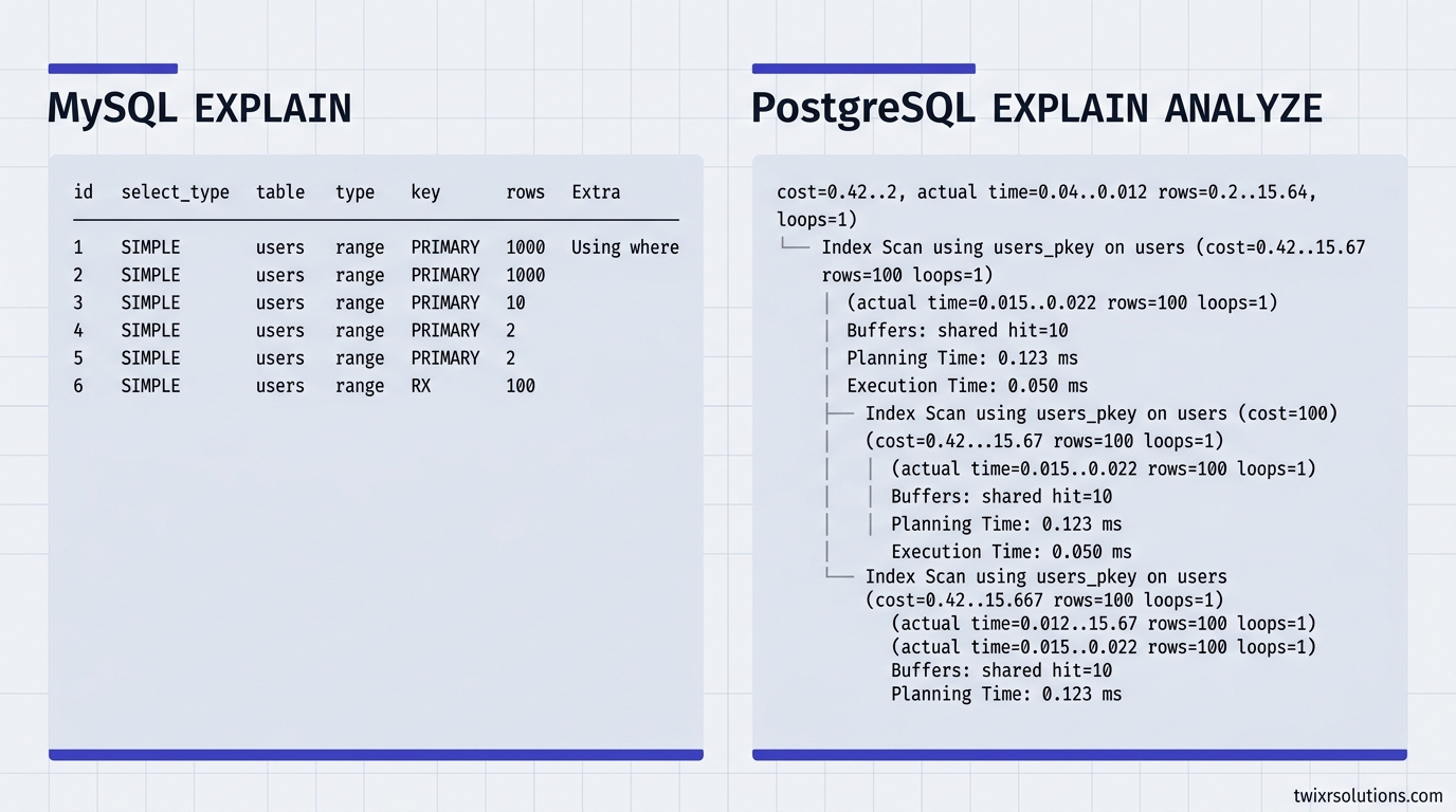
Reality: MySQL and PostgreSQL use different output formats, different node names, and different metrics.

In MySQL 8+, use EXPLAIN FORMAT=JSON or EXPLAIN ANALYZE (added in 8.0.18). The type column in MySQL's classic output maps to access method: ALL is a full table scan, ref is an index lookup by equality, range is a bounded index scan. eq_ref means one row per outer row - usually what you want in joins.

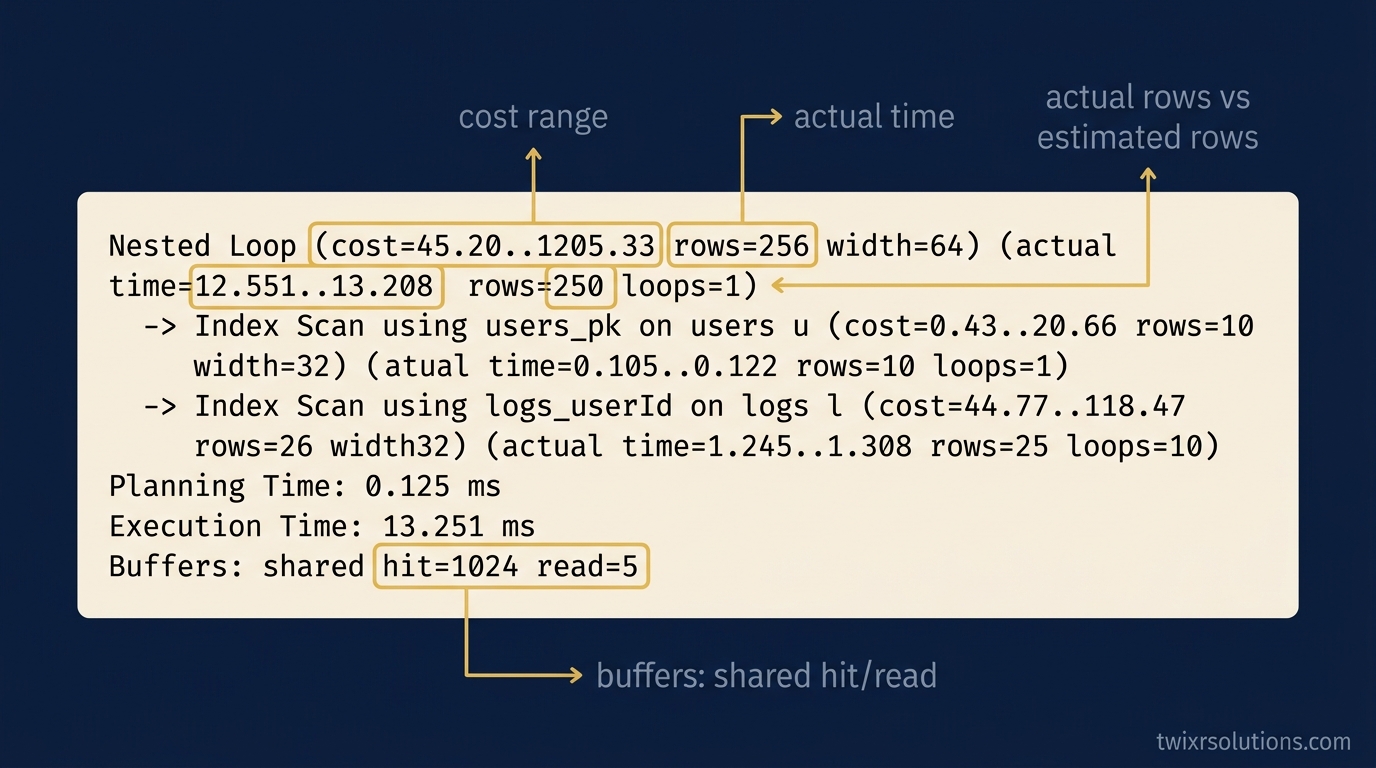
In Postgres, every node has cost, actual time, rows, and loops. The loops value multiplies actual time - a node that runs 500 times and costs 2ms per loop is adding 1 second, not 2ms. Always multiply.

---

Myth 5: "The slowest query is the one to fix first"

Reality: Fix the query that runs most often at a bad cost, not just the one-off that took the longest.

A 4-second query that runs twice a day costs 8 seconds. A 200ms query that runs 2,000 times a day costs 400 seconds. Your monitoring tool needs to show total_time, not just max_time.

In Postgres, pg_stat_statements gives you this:

SELECT query, calls, total_exec_time, mean_exec_time
FROM pg_stat_statements
ORDER BY total_exec_time DESC
LIMIT 10;

This is how you prioritize. Not by which query felt slow in staging.

---

A Practical Reading Sequence

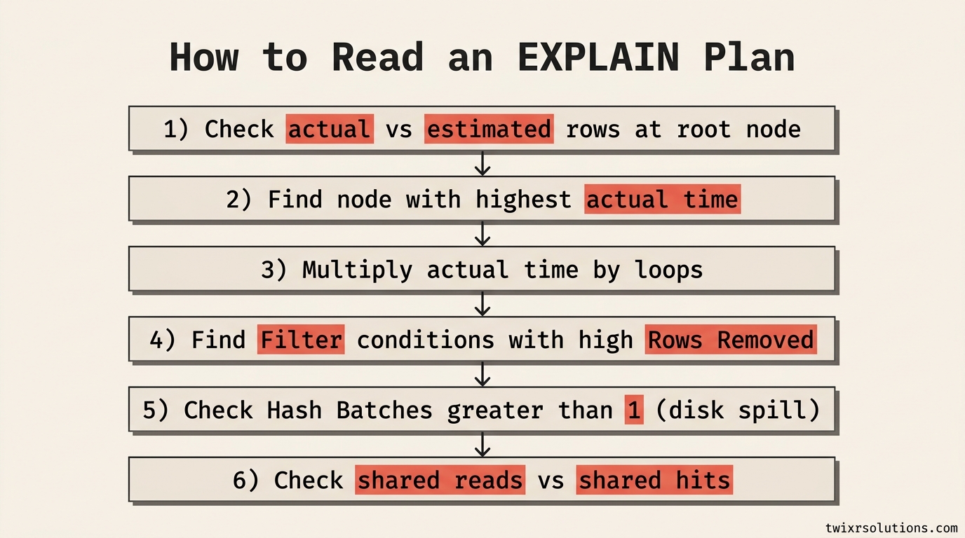
When you open an EXPLAIN plan, work through it in this order:

1. Check actual vs estimated rows at the top-level node. A large mismatch means bad statistics or a bad join condition.
2. Find the highest actual time node. That is where time is actually being spent.
3. Check loops. Multiply actual time by loops to get real cost.
4. Look for Filter conditions with high Rows Removed by Filter. Index is not selective enough.
5. Look for Hash Batches > 1. Hash join spilled to disk. Work_mem is too low for this query.
6. Check buffer hits vs reads. High shared read means data is not in cache.

Do not jump to indexing until you have done steps 1 through 3. Most premature indexes fix the wrong thing.

---

One Thing to Do Right Now

Run this against your Postgres database if you have pg_stat_statements enabled:

SELECT
  LEFT(query, 80) AS query_snippet,
  calls,
  ROUND(total_exec_time::numeric, 2) AS total_ms,
  ROUND(mean_exec_time::numeric, 2) AS avg_ms
FROM pg_stat_statements
WHERE calls > 50
ORDER BY total_exec_time DESC
LIMIT 5;

Take the top result. Run EXPLAIN (ANALYZE, BUFFERS) on it. Follow the six-step sequence above. You will almost always find something - a row estimate mismatch, a spilled hash join, or a filter eating rows your index missed.

That is how you stop guessing.